Building a Vector Database in Python

Introduction

Vector databases are fundamental to generative AI. They solve the hallucination challenge with LLMs by allowing us ground responses with correct information at inference time through Retrieval Augmented Generation. They are also used now to power advanced memory in agentic systems.

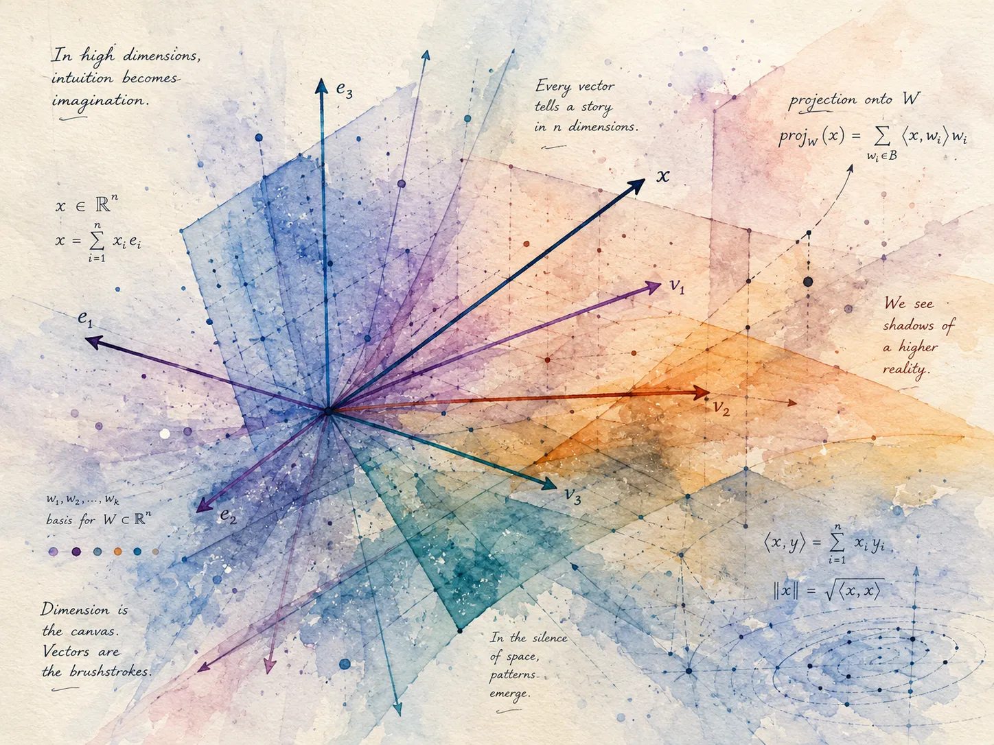
Watercolour illustration of vectors

For a long time they felt like magic to me, a black box you pip install, throw some text at, and somehow get back “similar” results. I don’t like black boxes, so I decided to build one from scratch as a learning project. I called it jvdb.

This article is not a polished step-by-step tutorial. It is more of a devlog, a writeup of the actual journey: the concepts I had to understand first, the two versions I built (a pure Python one and a NumPy one), the bugs and design problems I ran into, and what I measured when I finally profiled the thing. If you have ever wondered what is actually happening inside a vector database, I think building a tiny one yourself is the fastest way to find out.

Let’s get into it!

Some concepts I had to understand first

Before writing a single line of the database, I needed to get a few ideas straight in my head. If these are already familiar to you, feel free to skip ahead to Stage 1.

What even is a vector database?

A normal database stores rows and lets you query them by exact values: “give me every user where country = 'United Kingdom'”. That works great when you know exactly what you are looking for. But it falls apart the moment you want to search by meaning. If I store the sentence “Where is my money?” and later search for “I need my funds”, a normal WHERE clause finds nothing, because the words don’t match, even though the meaning is almost identical.

A vector database solves this. Instead of storing text and matching it character by character, it stores a numerical representation of the meaning of each piece of text, and lets you search by closeness in meaning. So the core job of a vector database is actually pretty narrow:

Take some data (text, in my case), turn it into vectors, and store them.
Given a query, turn the query into a vector too.
Find the stored vectors that are most “similar” to the query vector.
Return the original data behind those top matches.

That’s it. Everything else, persistence, deduplication, indexing, is a detail on top of those four steps.

Embeddings

So how do you turn “Where is my money?” into numbers? You use an embedding model. An embedding is a list of floating point numbers that represents the meaning of a piece of text as a point in space. Text with similar meaning ends up close together in that space, and text with different meaning ends up far apart.

I didn’t train my own embedding model (that is a whole other project), I used OpenAI’s embedding API:

def _generate_embeddings(self, input: str):
	response = self.client.embeddings.create(
		input=input,
		model=self.model
	)

	return response.data[0].embedding

You pass in a string, the model returns a list of floats. With text-embedding-3-small that list has 1536 numbers in it; with text-embedding-3-large, which I switched to later, it is even bigger. Each one of those numbers is a coordinate. So a single embedding is a point in 1536-dimensional space. I can’t picture 1536 dimensions and neither can you. But, a simpler example is a color as a point in a 3-dimensional space, with each RGB value as a dimension. So, black would be (0, 0, 0), white would be (255, 255, 255) and red would be (255, 0, 0), something like orange would be (255, 200, 152) which would be closer to red than black or white, both on the color spectrum and as points in a 3d space.

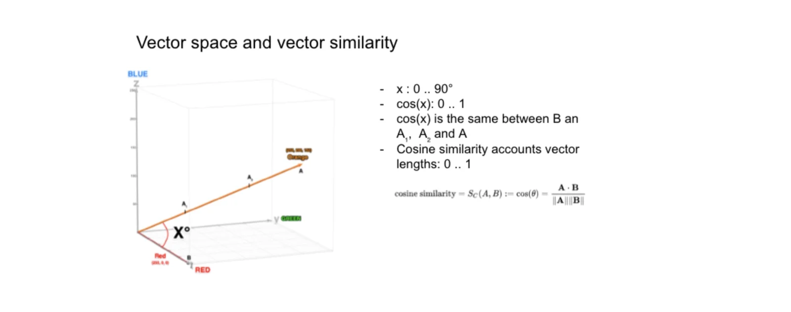Gloria Vinogradova, Vector search in old and modern databases

As you go beyond 3 dimensions it becomes harder to visualize higher dimensions on a cartesian plane. I asked Claude to visualize features of movies in a 6d space and this is what it looks like.

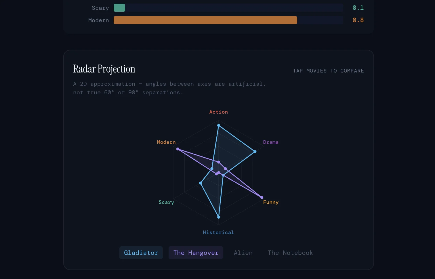Claude-generated diagram visualizing movie features in a 6D space Claude-generated diagram: https://claude.ai/chat/7d4efe68-8a5e-49c3-bc3c-db275212bb12

Visualizing higher dimensions is best done as a histogram (Claude taught me!) where each bar corresponds to a dimension.

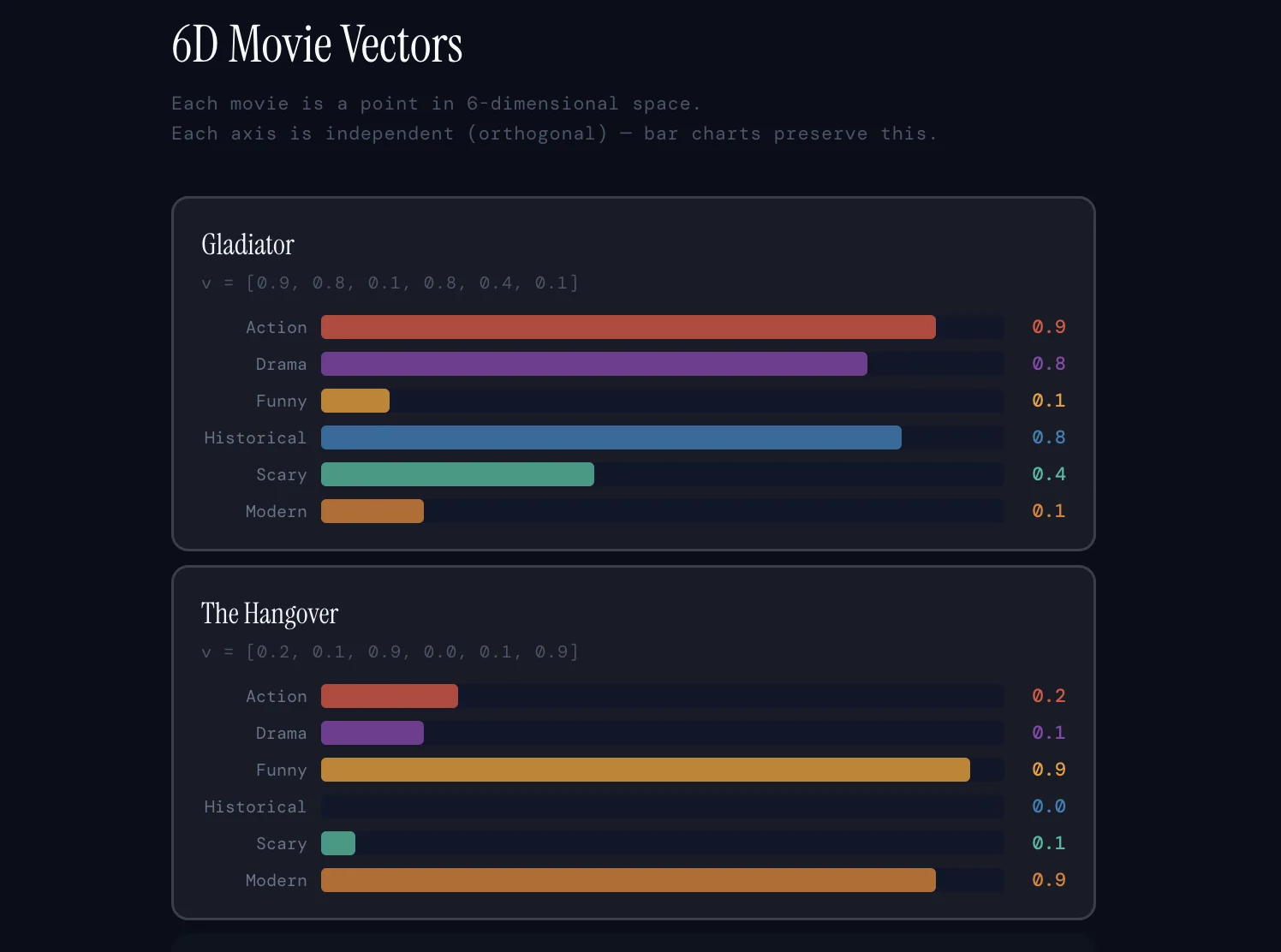Claude-generated histogram with one bar per dimension Claude-generated diagram: https://claude.ai/chat/7d4efe68-8a5e-49c3-bc3c-db275212bb12

Similarity

Once your text is a point in space, “find similar text” becomes “find nearby points”. The measure I used is cosine similarity, which compares the direction two vectors point in rather than how long they are.

The intuition I keep coming back to: imagine two arrows starting at the same origin. If they point in almost the same direction, they are similar (cosine close to 1). If they point in completely different directions, they are not (cosine close to 0). The formula is:

cosine_similarity = dot_product(a, b) / (norm(a) * norm(b))

Where the dot product multiplies matching positions and adds them up, and the norm is just the length of a vector (the straight-line distance from the origin). For a vector like [3, 4], the norm is sqrt(3² + 4²) = sqrt(25) = 5.

There is a lovely shortcut hiding in that formula, and it became the backbone of my NumPy version. If you normalize every vector first, meaning you divide it by its own length so its new length is exactly 1, then norm(a) * norm(b) becomes 1 * 1 = 1, and the whole thing collapses to:

cosine_similarity == dot_product(a, b)

So if I normalize my embeddings once, up front, then similarity search is just a dot product. No division per comparison. I’ll come back to why that matters so much for speed.

Storage: in-memory vs persistent

Here is a question I didn’t think about until I had a working prototype: where do the vectors actually live? The simplest answer is in-memory: keep everything in a Python list or a NumPy array inside the running process. It is fast and super simple, but the moment your program exits, everything is gone. Every time you restart, you have to re-embed all your data, which means paying for API calls again and waiting again. For a toy this is fine. For anything real it is not.

The other option is persistent storage: write the vectors to disk so they survive a restart. You generate the embeddings once, save them, and load them back the next time you start up. This is the difference between Stage 1 and Stage 2 of my project, and getting persistence right turned out to be more fiddly than I expected.

Python lists vs NumPy arrays for the embeddings

My first version stored everything in plain Python lists. It worked. It was also slow, and I had a hunch about why, which led me down a rabbit hole that I think is one of the most valuable things I learned in this whole project.

A Python list is incredibly flexible. You can put anything in it:

items = ["hello", 42, True, [1, 2, 3]]

A NumPy array is the opposite. It (usually) holds exactly one type of value:

import numpy as np

vector = np.array([0.1, 0.2, 0.3], dtype=np.float32)

That restriction looks like a downside but it is actually the entire reason NumPy is fast. Because NumPy knows every element is, say, a 32-bit float, it can hand the work off to heavily optimized C and BLAS routines and run math across the whole array at once, instead of looping in Python one element at a time. For a vector database, where the core operation is “multiply one query against thousands of stored vectors”, this is the difference between a toy and something usable.

Memory allocation: how Python stores data vs how NumPy stores data

This is the part that made everything click for me, so I want to spend some time explaining it.

When you put floats in a Python list, you are not storing the numbers themselves in a neat row. A Python list stores pointers to objects. Every single float is a full-blown Python object sitting somewhere on the heap, carrying a reference count, a type pointer, and the actual value, which adds up to roughly 24 bytes per number before you even count the pointer in the list. Worse, those objects can be scattered all over memory. So when you loop over a list of floats to add them up, the CPU is constantly chasing pointers to random addresses, and it can’t take advantage of the fast, predictable access patterns modern hardware is built for.

A NumPy array is the opposite. It stores the raw numbers themselves, packed tightly together in one contiguous block of memory, with no per-number Python object overhead. A float32 is exactly 4 bytes, sitting right next to the next 4 bytes, and so on. This does two things: it uses far less memory, and it lets the CPU stream through the data efficiently (and lets NumPy use vectorized CPU instructions under the hood).

You can see the memory part concretely. An embedding matrix of 10,000 documents with 1536 dimensions each, stored as float32:

embeddings.nbytes # 61,440,000 bytes == 58.59 MB

The same matrix as float64 (the default if you don’t specify):

embeddings.astype(np.float64).nbytes # 122,880,000 bytes == 117.19 MB

Exactly double, because each number went from 4 bytes to 8. That is why I store my embeddings as float32, the precision is more than enough for similarity search, and it halves the memory. Compare either of those to a Python list of lists of floats, where the per-object overhead would balloon the same data into hundreds of megabytes, and you start to see why I ultimately decided to implement a Numpy version of jvdb for the second part of the project.

Stage 1: an in-memory vector store in pure Python

My first goal was just to get the four steps working with zero magic and zero dependencies beyond the OpenAI client. No NumPy, no persistence, just Python lists and loops. The whole thing lived in a class called VectorDB:

class VectorDB:

	def __init__(self, data: list[str]):
		self.data = data
		self.store = []
		_client = OpenAI(api_key=os.environ['OPENAI_API_KEY'])

self.data is the list of raw texts I want to search through, and self.store is where I’ll keep each text paired with its embedding. I embedded the stored texts by looping over them and storing each text-and-embedding pair as a dictionary:

def _generate_embeddings_for_stored_texts(self):

	for text in self.data:
		temp_map = {}
		embeddings = self._generate_embeddings(text)
		temp_map["text"], temp_map["embeddings"] = text, embeddings
		self.store.append(temp_map)

So self.store ends up looking like this:

[
	{"text": "I am fine", "embeddings": [0.01, -0.04, ...]},

	{"text": "The capital of the United Kingdom is London", "embeddings": [...]},

	{"text": "Where is my money?", "embeddings": [...]},
]

Then came the math. Since I wasn’t using NumPy yet, I had to write cosine similarity by hand, from the ground up. First the magnitude (norm) of a vector:

def _magnitude(self, vector: list[float]) -> float:

	sum_squares = 0

	for point in vector:
		square = point * point
		sum_squares += square
		mag = math.sqrt(sum_squares)

	return mag

This is the textbook definition: square every component, add them up, take the square root. Then the dot product, which walks two vectors in lockstep, multiplying matching positions and accumulating the total:

def _dot_product(self, vector_1: list[float], vector_2: list[float]) -> float:

	dp = 0

	for point_1, point_2 in zip(vector_1, vector_2):
		product = point_1 * point_2
		dp += product

	return dp

And finally cosine similarity, which just glues the two together with the formula from earlier:

def _cosine_similarity(self, vector_1: list[float], vector_2: list[float]) -> float:

	vector_1_magnitude, vector_2_magnitude = self._magnitude(vector_1), self._magnitude(vector_2)
	dot_product_of_vectors = self._dot_product(vector_1, vector_2)
	cs_numerator = vector_1_magnitude * vector_2_magnitude
	cs = dot_product_of_vectors / cs_numerator

	return cs

Writing this by hand was genuinely worth it. I had read the cosine similarity formula a dozen times before, but implementing every loop yourself forces you to actually understand it.

Search ties it all together: embed the query, score every stored item against it, sort by score, return the top k:

def search(self, query_text: str, k: int):

	matches = []
	query = self._generate_embeddings_for_query_text(query_text)
	query_embeddings = query["embeddings"]
	self._generate_embeddings_for_stored_texts()

	store_copy = [item for item in self.store]

	for item in store_copy:
		embedding = item["embeddings"]
		cs_score = self._cosine_similarity(query_embeddings, embedding)
		item["score"] = cs_score

	def _cosine_score(item: dict):

		return item["score"]
		store_copy.sort(key=_cosine_score, reverse=True)

	for item in store_copy[:k]:

		matches.append({"text": item["text"], "score": item["score"]})

	return matches

This worked, and the first time I ran it and got back semantically relevant results instead of keyword matches, and I felt a great sense of accomplishment and satisfaction.

But look closely at that search method and you can spot the design flaw that sent me to stage 2: self._generate_embeddings_for_stored_texts() is called inside search. That means every single search re-embeds every stored document, hitting the OpenAI API again and again for data that hasn’t changed. It’s slow, it costs money, and it scales terribly. The fix is to separate “build the store once” from “search the store many times”, and that realization is what pushed me toward a proper, persistent, NumPy-based version.

Stage 2: a persistent vector store with NumPy

Stage 2 is the version I actually like. It does three things Stage 1 didn’t: it stores embeddings in a NumPy array instead of a list of dicts, it persists everything to disk so I never re-embed the same text twice, and it has a small CLI so I can use it like a real tool. The class lives in db.py.

It starts by deciding where data lives on disk:

JVDB_HOME = Path.home() / ".jvdb"
DATASTORE_DIR = JVDB_HOME / "datastore"
DATASTORE_DIR.mkdir(parents=True, exist_ok=True)

class VectorDB:

	def __init__(self, name: str):
		self.name = name
		self.data_file_name = DATASTORE_DIR / f"{self.name}.data.json"
		self.emb_file_name = DATASTORE_DIR / f"{self.name}.emb.npz"
		self.data = self.load_from_disk(self.data_file_name)
		self.hashed_data = self._hash_data_items()
		self.embeddings = self.load_from_disk(self.emb_file_name)
		self.client = OpenAI(api_key=os.environ["OPENAI_API_KEY"])
		self.model = "text-embedding-3-large"

Two decisions here that I’m happy with. First, each named database gets its own pair of files under ~/.jvdb/datastore/: a .data.json for the texts and a .emb.npz for the embeddings. Second, the texts and the embeddings are stored separately. The text is human-readable string data that belongs in JSON; the embeddings are a big block of numbers that belongs in NumPy’s own format. They are linked purely by position, the row at index i in the embeddings array corresponds to the item at index i in the data list. (More on how easy it is to break that link in the Challenges section.)

The key change from Stage 1 is how similarity search works. Because I normalize every embedding when I store it, search becomes a single matrix-vector multiplication:

def _cosine_similarity(self, vector_embs, query_emb) -> list[float]:
	result = vector_embs @ query_emb
	return result

That @ operator is matrix multiplication. vector_embs is the whole stored matrix with shape (number_of_documents, dimensions), and query_emb is a single normalized query vector. The result is one similarity score per stored document, computed in one shot, in optimized C, instead of a Python loop calling _cosine_similarity thousands of times. The entire scoring step of Stage 1 collapses into one line.

Search then normalizes the query, scores everything, and grabs the top k using argsort:

def search(self, query, k: int):

	if self._validation_checks() is False:
		return

	if k < 1:
		raise ValueError("number of matches cannot be less than 1.")

	if k > len(self.embeddings) or k > len(self.data):
		raise ValueError("number of matches cannot be more than number of records.")

	vector_embs = self.embeddings
	query_emb = self._normalize_query_embeddings(query)
	similarity_scores = self._cosine_similarity(vector_embs, query_emb)
	sorted_scores_indices = np.argsort(similarity_scores)[::-1][:k]

	top_k_matches = []

	for index in sorted_scores_indices:
		top_k_matches.append({
		"text": self.data[index],
		"score": float(similarity_scores[index])
		})

	return top_k_matches

np.argsort(similarity_scores) returns the indices that would sort the scores in ascending order; [::-1] reverses it to descending; [:k] takes the top k. I argsort the indices rather than the scores themselves precisely because the index is the thread connecting a score back to its text in self.data. Sort the scores directly and you lose that thread entirely.

For persistence, saving writes the two files in their respective formats:

def save_to_disk(self):
	data_path = Path(self.data_file_name)
	emb_path = Path(self.emb_file_name)

	with open(data_path, "w+") as f:
		json.dump(self.data, f)

	np.savez_compressed(emb_path, self.embeddings)

	return {"message": f"saved data and embeddings to {data_path}, {emb_path} respectively."}

I went back and forth on this. I originally tried dumping the embeddings into JSON too, but storing a giant array of floats as text is wasteful and slow to parse. np.savez_compressed stores the array in NumPy’s native binary format and compresses it, which is far better suited to a big block of numbers. Loading mirrors it, returning an empty list if the file doesn’t exist yet so a brand-new database just starts empty:

def load_from_disk(self, filename):

	path = Path(filename)

	if not path.exists():
		return []

	if ".npz" in path.name:
		data = np.load(path)
		return data["arr_0"]

	with open(path, "r+") as f:
		data = json.load(f)
	return data

Finally, a small argparse CLI turns this into something I can actually run from a terminal:

def main():

	parser = argparse.ArgumentParser(prog="jvdb")

	parser.add_argument(
		"--db",
		default="default",
		help="database name to use"
	)

	subparsers = parser.add_subparsers(dest="command", required=True)
	insert_parser = subparsers.add_parser("insert")
	insert_parser.add_argument("text")

	search_parser = subparsers.add_parser("search")
	search_parser.add_argument("query")
	search_parser.add_argument("-k", type=int, default=2)

	args = parser.parse_args()

	db = VectorDB(name=args.db)

	if args.command == "insert":
		db.insert(args.text)

	elif args.command == "search":
		results = db.search(args.query, k=args.k)

	for result in results:
		print(result)

I turned jvdb into a uv package that I could run from anywhere on my laptop locally, here is what a result looks like:

Challenges I faced

Keeping indexes aligned across data and embeddings

The single biggest source of bugs in the whole project was this: my texts live in a Python list (and a JSON file), and my embeddings live in a NumPy array (and an .npz file). Nothing in the code physically ties row 5 of the embeddings to item 5 of the texts. They are linked only by position, by a silent convention that I have to maintain perfectly everywhere.

If I ever append an embedding without appending the matching text, or load one file successfully and the other partially, or sort one without the other, the two drift out of alignment, and the database doesn’t crash. It quietly returns the wrong text for the right score. That is the worst kind of bug, because everything looks like it’s working.

I ended up adding a guard that runs before every search to at least catch the obvious case:

def _validation_checks(self):

	if len(self.embeddings) != len(self.data):
		print("embeddings and data are not the same length. mismatched index.")
		return False

	elif len(self.data) != np.shape(self.embeddings)[0]:
		print("embeddings rows != data rows. mismatched index.")
		return False

	else:
		return True

It checks that the number of texts equals the number of embedding rows before it trusts the data enough to search it. It is not a complete solution, two lists can be the same length and still be misaligned internally, but it caught real mistakes while I was developing, and it taught me an important lesson: when your data is split across parallel structures, the alignment between them is itself a thing you have to actively protect. A more mature design would bundle each text and its vector together with a shared ID so they can’t drift apart, and that is high on my list of things to refactor.

Upserting to the vector store

The second challenge was inserting new data without creating a mess. I wanted insert to do the obvious right thing: add genuinely new text, but skip text I already have, so re-running the same insert doesn’t fill my database with duplicates. That “insert or update, but don’t duplicate” behaviour is what people in the database field call an upsert.

The naive way to check for duplicates is to compare the new text against every stored text one by one, which is an O(n) scan on every insert. Instead I hash each text and keep the hashes in a dictionary, so checking for a duplicate is an O(1) lookup. I used blake2b for a stable hash:

def _stable_hash(self, text: str) -> int:

	digest = blake2b(text.encode("utf-8"), digest_size=8).digest()
	hash = int.from_bytes(digest, "little", signed=False)
	return hash

The word “stable” matters here. Python’s built-in hash() is randomized between runs for security reasons, so the same string gives a different number every time you restart the program, which is useless if you want to persist hashes to disk and compare across sessions. blake2b always returns the same digest for the same input, so it survives restarts. When the database loads, it rebuilds a map of every existing hash:

def _hash_data_items(self):
	hash_data_map = {}

	for item in self.data:
		item_hash = self._stable_hash(item["content"])
		hash_data_map[item_hash] = item

	return hash_data_map

def is_dup(self, new_data) -> bool:
	new_data_hash = self._stable_hash(new_data)
	return new_data_hash in self.hashed_data

And insert puts it all together: bail early if it’s a duplicate, otherwise embed the new text, normalize it, and append it to the matrix:

def insert(self, new_data: str):

	if self.is_dup(new_data):
		print("Duplicate item. Skipping upsert.")
	return

	new_data_embeddings = np.array([self._generate_embeddings(new_data)], dtype=np.float32)

	new_data_embeddings = self._normalize(new_data_embeddings, self._norm(new_data_embeddings, axis=1))

	if len(self.embeddings) == 0:
		self.embeddings = new_data_embeddings
	else:

		self.embeddings = np.vstack([self.embeddings, new_data_embeddings])
		data_dict = {"id": len(self.data), "content": new_data}
		self.data.append(data_dict)
		new_data_hash = self._stable_hash(new_data)
		self.hashed_data[new_data_hash] = new_data

	self.save_to_disk()

Two things in here bit me and are worth flagging. First, that if len(self.embeddings) == 0 branch is not optional. NumPy is fussy about shapes, and trying to vstack a new row onto a freshly-loaded empty array throws a shape error, so the very first insert into a brand-new database has to be handled as a special case. Second, notice how many things have to be appended together in the right order: the embedding row, the data dict, and the hash entry. This is exactly the index-alignment problem from the last section showing up in practice. Every insert is a tiny opportunity to desync my three structures, which is why getting insert correct took me several commits of “fixed embeddings storage bugs” before I trusted it.

Profiling: how much faster is NumPy, really?

I had a strong intuition that the NumPy version was faster, but intuition isn’t a number, so I profiled it. I wanted to answer one question: for the core similarity search, how much does NumPy actually buy me over my hand-written Python loops?

The right way to benchmark this is to not include the embedding API calls. Network latency would completely dominate the timing and drown out the thing I actually care about, so I followed the local-benchmark approach: generate fake random embeddings, then time only the scoring and sorting. I used 10,000 documents with 1536 dimensions each, the same shape as a real text-embedding-3-small store:

NUM_DOCS, DIM = 10_000, 1536
rng = np.random.default_rng(42)
embeddings = rng.random((NUM_DOCS, DIM), dtype=np.float32)
query = rng.random(DIM, dtype=np.float32)

For benchmarking I reached for cProfile, Python’s built-in profiler. The simplest way to use it is cProfile.run(), which takes a string of code to execute and prints a table of where the time went:

import cProfile
	cProfile.run("search_pure_python(5)", sort="cumulative")
	cProfile.run("search_numpy(5)", sort="cumulative")

Here is the result for the pure Python version, the one using my _magnitude and _dot_product loops:

40007 function calls in 0.849 seconds

ncalls tottime percall cumtime percall filename:lineno(function)

1 0.000 0.000 0.849 0.849 search_pure_python

10000 0.503 0.000 0.503 0.000 _dot

10001 0.333 0.000 0.334 0.000 _magnitude

1 0.003 0.003 0.003 0.003 {method 'sort' of 'list' objects}

And here is the NumPy version, doing the exact same search:

9 function calls in 0.002 seconds

ncalls tottime percall cumtime percall filename:lineno(function)

1 0.000 0.000 0.002 0.002 search_numpy

1 0.000 0.000 0.001 0.001 {method 'argsort' of 'numpy.ndarray' objects}

The pure Python search took about 832 ms. The NumPy search took about 2 ms. That is roughly a 400x speedup for the same logical operation on the same data. And cProfile tells you exactly where the Python version spends its life: 10,000 calls to _dot (0.5s) and 10,001 calls to _magnitude (0.33s). Those two pure-Python loops are essentially the entire runtime. The NumPy version makes a grand total of 9 function calls, because the heavy lifting happens down in C where the profiler can’t even see it.

This is the memory story from the introduction made visible. The Python version is chasing scattered pointers and interpreting bytecode 1536 numbers at a time, ten thousand times over. The NumPy version streams through one contiguous 58 MB block and lets BLAS do the multiply. Seeing that 832 ms versus 2 ms with my own eyes was the most satisfying moment of the whole project, because it turned a vague “NumPy is faster” into a concrete, measured fact I could explain.

(As an aside, cProfile.run() is the quick way in, but if you want to profile a real method without wrapping it in a string, you can use a cProfile.Profile() object directly, enable and disable it around the call, and dump the stats with pstats. I wrapped that pattern in a small decorator so I could sprinkle @profile_function on anything I wanted to inspect.)

Next steps: more efficient indexing

Right now jvdb does what is called a flat or brute force search: every query is compared against every stored vector. My profiling shows that, thanks to NumPy, this is shockingly fast even at 10,000 documents, a couple of milliseconds. But it is still fundamentally O(n). Double the documents and you double the work. At 10,000 vectors that’s invisible; at 10 million it is not, and a single matrix that big may not even fit comfortably in memory.

The first, easiest win is to stop fully sorting the scores. I currently use np.argsort(scores)[::-1][:k], which sorts all 10,000 scores just to take the top 5. NumPy has np.argpartition, which finds the top k without fully ordering everything else:

top_indexes_unsorted = np.argpartition(scores, -k)[-k:]

top_indexes = top_indexes_unsorted[np.argsort(scores[top_indexes_unsorted])[::-1]]

That is a nice constant-factor improvement, but it is still O(n) at heart, it still touches every score.

The real next step, and the thing I want to learn next, is approximate nearest neighbour (ANN) indexing. Instead of comparing the query to every vector, you build a smart index ahead of time that lets you skip most of them, trading a tiny bit of accuracy for an enormous speedup. The most popular approach is HNSW (Hierarchical Navigable Small World graphs), which is what production vector databases like FAISS, Qdrant, and pgvector use under the hood. The idea is to organise the vectors into a layered graph you can navigate towards the query’s neighbourhood in roughly logarithmic time instead of linear.

That is a meaty enough topic to be its own project, and honestly its own article. Building the brute force version first was the right call, though: I now understand exactly what problem an ANN index is solving, because I’ve felt the O(n) cost myself and watched it in the profiler.

Conclusion

I set out to demystify vector databases for myself, and building jvdb was very challenging and fundamentally taught me the important concepts on vector databases. The headline lesson is that a vector database is conceptually simple, embed, store, compare by similarity, return the top matches, but the engineering details are where all the learning hides: choosing between in-memory and persistent storage, understanding why NumPy’s contiguous arrays crush Python lists for numeric work, keeping parallel data structures in alignment, making upserts idempotent, and proving your performance assumptions with a profiler instead of guessing.

If you have only ever used vector databases as a black box, I really do recommend building a tiny one. Start with the pure Python version, even though it’s “wrong”, because writing cosine similarity by hand teaches you the math, then rebuild it with NumPy and persistence and feel the difference. You will come away understanding not just how to use these tools, but why they are built the way they are.

You can find all the code for jvdb here: https://github.com/Chinenyay/jvdb. It’s a little messy because my entire learning process is literally recorded there: my notes, little functions I wrote to understand stuff before adding them to the project and the python lists and numpy ndarray versions.

I’ll be writing up the ANN/HNSW version once I’ve built it, so if you enjoyed this one, stay tuned!

Till another time,

Jennifer